
In my previous post, I introduced the Variational Autoencoder, a type of generative model. In this post, I will continue the discussion by exploring another prominent type of generative model: the diffusion model. Diffusion models have shown great promise in image synthesis, producing high-quality and high-fidelity images. Recent successful works such as Stable Diffusion, DALL-E, and Imagen have been shown that Diffusion models are also able to achieve consistent image-text alignment in text-to-image synthesis.
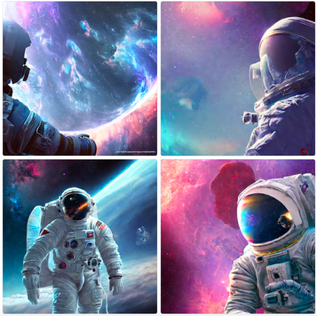 Fig 1. Samples generated by Stable Diffusion (source: Stable Diffusion)
In Section 1, I’ll delve into how diffusion works; Then, I’ll demonstrate how diffusion models can be applied to text-to-image synthesis in Section 2.
Diffusion models
Diffusion models work by gradually injecting noise into data and then learning to reverse this process. They are mostly based on three predominant formulations: denoising diffusion probabilistic models (DDPMs), score-based generative models (SGMs), and stochastic differential equations (Score SDEs).
In this post, I concentrate on DDPMs cause the most recent successful works are based on DDPMs and indeed they are fast and easy to train than other methods.
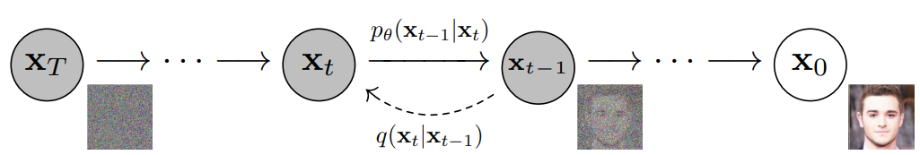 Fig 2. Denosing diffusion probabilistic models (source: Ho et al.)
Forward process
Forward process or diffusion process corrupts data (e.g. images) by gradually adding noise through number of timesteps $T$. From an image from real data distribution $x_0 \sim q(x)$, we can easily generate a sequence of noisy images $x_1, \dots, x_T$ through the diffusion process.
This process can be represented as a Markov chain that adds Gaussian noise into data step by step with a pre-determined variance schedule $\beta_1, \dots, \beta_T$:
\[\begin{align} q(\mathbf{x}_{1:T} \vert \mathbf{x}_0) &= \prod^T_{t=1} q(\mathbf{x}_t \vert \mathbf{x}_{t-1}) \notag\\ q(\mathbf{x}_t \vert \mathbf{x}_{t-1}) &= \mathcal{N}(\mathbf{x}_t; \sqrt{1 - \beta_t} \mathbf{x}_{t-1}, \beta_t\mathbf{I}), \end{align}\]where \(q(\mathbf{x}_t \vert \mathbf{x}_{t-1})\) is known as forward diffusion kernel (FDK), and we use Normal/Gaussian distribution to define this term. Hence, at each timestep $t$, the parameters that define the distribution of image $x_t$ are set as:
- Mean: $\sqrt{1 - \beta_t}x_{t-1}$
- Covariance: $\beta_t\mathbf{I}$.
🤓 Note:
\[\begin{equation} q(\mathbf{x}_t \vert \mathbf{x}_0) = \mathcal{N}(\mathbf{x}_t; \sqrt{\bar{\alpha}_t} \mathbf{x}_0, (1 - \bar{\alpha}_t)\mathbf{I}) \end{equation}\]
- $\sqrt{1 - \beta_t}$ is used in a diffusion process because it provides a smooth transition from the original state of the data to the noisy state. It ensures that the amount of noise that is added to the data is gradual and does not suddenly increase.
- The term $\mathbf{I}$ is an identity matrix. Therefore, the distribution at each time step is called Isotropic Gaussian.
- Instead of gradually computing $x_0, \dots, x_{t−1}$ to sample $x_t$, we can use the reparameterization trick to compute $x_t$ directly, with \(\alpha_t = 1 - \beta_t\) and \(\bar{\alpha}_t = \prod_{i=1}^t \alpha_i\):
“By choosing sufficiently large timesteps and defining a well-behaved schedule of $\beta_t$ the repeated application of FDK gradually converts the data distribution to be nearly an Isotropic Gaussian distribution.” - Vaibhav Singh, 2023
Backward process
The true power of diffusion models lies in their ability to reverse the diffusion process. To generate a true sample from a Gaussian noise input, \(\mathbf{x}_T \sim \mathcal{N}(\mathbf{0}, \mathbf{I})\), we can reverse the forward process by sampling from \(q(\mathbf{x}_{t-1} \vert \mathbf{x}_t)\) until we obtain \(q(\mathbf{x}_0)\). This reverse process is known as the joint distribution \(p_\theta(\mathbf{x}_{0:T})\). However, since \(q(\mathbf{x}_{t-1} \vert \mathbf{x}_t)\) is intractable, we need to learn a model \(p_\theta\) to approximate these conditional probabilities in order to run the reverse diffusion process. Thus, the reverse process is defined as a Markov chain with \(p_\theta\):
\[\begin{align} p_\theta(\mathbf{x}_{0:T}) &= p(\mathbf{x}_T) \prod^T_{t=1} p_\theta(\mathbf{x}_{t-1} \vert \mathbf{x}_t) \notag\\ p_\theta(\mathbf{x}_{t-1} \vert \mathbf{x}_t) &= \mathcal{N}(\mathbf{x}_{t-1}; \boldsymbol{\mu}_\theta(\mathbf{x}_t, t), \boldsymbol{\Sigma}_\theta(\mathbf{x}_t, t)) \end{align}\]where \(p_\theta(\mathbf{x}_{t-1} \vert \mathbf{x}_t)\) is known as the reverse diffusion kernel (RDK). Just like the FDK, we can define the reverse diffusion kernel using a Normal/Gaussian distribution. This process can start with $p(x_T)=\mathcal{N}(\mathbf{x}_t; 0, \mathbf{I})$ since $q(x_T) \approx \mathcal{N}(\mathbf{x}_t; 0, \mathbf{I})$ at the end of the forward process.
🤓 Note: $p(x_T)$ doesn’t need learnable parameter $\theta$ because $x_T$ is a Gaussian noise.
Finally, we obtain this process objective $p_\theta(x_0)$ by integrating over a very high dimensional (pixel) space for continuous values over $T$ timestep:
\[p_\theta(x_0)=\int{p_\theta(x_{0:T})}dx_{1:T}\]Intuitively, we have to integrate over all “pathways” from a pure noise $x_T$ to reach a data sample $x_0$. And certainly, this is an extremely complex computing process ☠️. However, we can use a technique called VLB to optimize $p_\theta(x_0)$ instead of explicitly computing it through integration. We will discuss this in more detail in the next section.
Training objective and Loss function
The training objective of our diffusion model is minimizing the negative log-likelihood probability of the sample generated $p_\theta(x_0)$ belonging to the same data distribution as the original data. So, the loss function for training our neural network amounts to:
\[L = -\log p_\theta(x_0)\]As we already know, this term is intractable due to the need to perform integration over a high-dimensional pixel space. To overcome this challenge, we use a Variational Lower Bound (VLB), also known as Evidence Lower Bound (ELBO) to optimize the negative log-likelihood, similar to the approach used in Variational Autoencoders (VAEs).
\[\begin{aligned} L_\text{VLB} &= \mathbb{E}_{q(\mathbf{x}_{0:T})} \Big[ \log \frac{q(\mathbf{x}_{1:T}\vert\mathbf{x}_0)}{p_\theta(\mathbf{x}_{0:T})} \Big] \geq - \mathbb{E}_{q(\mathbf{x}_0)} \log p_\theta(\mathbf{x}_0) \end{aligned}\]By rewriting the objective as a combination of several KL-divergence and entropy terms (see the detailed step-by-step process in Appendix A in Ho et al., 2020, the objective becomes:
\[L_\text{VLB} = \mathbb{E}_q [\underbrace{D_\text{KL}(q(\mathbf{x}_T \vert \mathbf{x}_0) \parallel p_\theta(\mathbf{x}_T))}_{L_T} + \sum_{t=2}^T \underbrace{D_\text{KL}(q(\mathbf{x}_{t-1} \vert \mathbf{x}_t, \mathbf{x}_0) \parallel p_\theta(\mathbf{x}_{t-1} \vert\mathbf{x}_t))}_{L_{t-1}} \underbrace{- \log p_\theta(\mathbf{x}_0 \vert \mathbf{x}_1)}_{L_0} ]\]Let’s break it down into smaller segments:
\[\begin{aligned} L_\text{VLB} &= L_T + L_{T-1} + \dots + L_0 \\ \text{where } L_T &= D_\text{KL}(q(\mathbf{x}_T \vert \mathbf{x}_0) \parallel p_\theta(\mathbf{x}_T)) \\ L_t &= D_\text{KL}(q(\mathbf{x}_t \vert \mathbf{x}_{t+1}, \mathbf{x}_0) \parallel p_\theta(\mathbf{x}_t \vert\mathbf{x}_{t+1})) \text{ for }1 \leq t \leq T-1 \\ L_0 &= - \log p_\theta(\mathbf{x}_0 \vert \mathbf{x}_1) \end{aligned}\]Due to the work of Ho et al., this term has been simplified as we can now ignore $L_0$ and $L_T$:
- $L_0$: Empirical evidence from their work suggests that better results were achieved without the inclusion of $L_0$.
- $L_T$: is constant and can be ignored during training because $q$ does not have any learnable parameters and $x_T$ is a Gaussian noise.
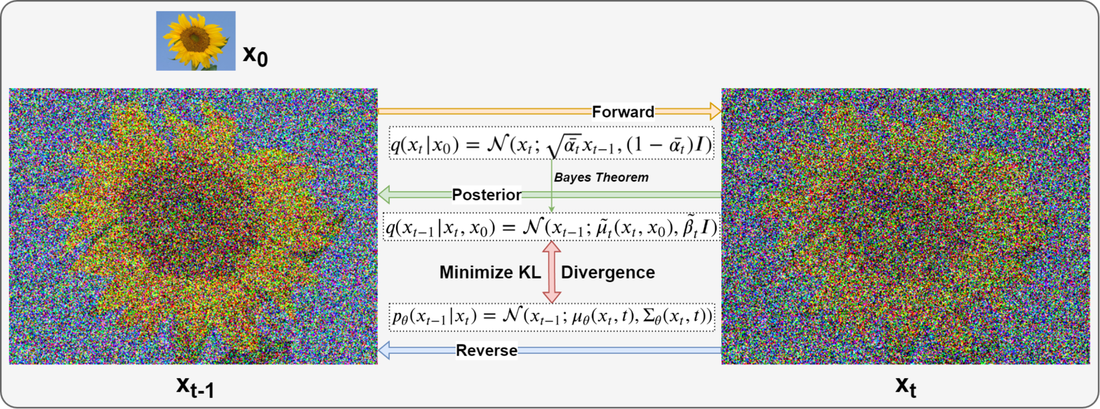 Fig 3. Training objective (source: learnopencv)
The only term that requires attention is $L_t$. To minimize the KL divergence, we must learn a neural network that can approximate the conditioned probability distributions in the reverse diffusion process:
\[q(\mathbf{x}_{t-1} \vert \mathbf{x}_t, \mathbf{x}_0) = \mathcal{N}(\mathbf{x}_{t-1}; \color{blue}{\tilde{\boldsymbol{\mu}}}(\mathbf{x}_t, \mathbf{x}_0), \color{red}{\tilde{\beta}_t} \mathbf{I})\]where \(\color{blue}{\tilde{\boldsymbol{\mu}}_t=\frac{1}{\sqrt{\alpha_t}} \Big( \mathbf{x}_t - \frac{1 - \alpha_t}{\sqrt{1 - \bar{\alpha}_t}} \boldsymbol{\epsilon}_t \Big)}\) and \(\color{red}{\boldsymbol{\tilde{\beta}}_t=\frac{1 - \bar{\alpha}_{t-1}}{1 - \bar{\alpha}_t} \cdot \beta_t}\) (see the detailed step-by-step process in Lilianweng’s blog). Namely, our network must be trained to approximate the parameters of the Gaussian distribution ($\color{blue}{\tilde{\boldsymbol{\mu}}_t}$ and $\color{red}{\boldsymbol{\tilde{\beta}}_t}$):
\[p_\theta(\mathbf{x}_{t-1} \vert \mathbf{x}_t) = \mathcal{N}(\mathbf{x}_{t-1}; \color{blue}{\boldsymbol{\mu}_\theta(\mathbf{x}_t, t)}, \color{red}{\boldsymbol{\Sigma}_\theta(\mathbf{x}_t, t)})\]In order to simplify the model’s task, the authors of DDPMs chose to fix the variance to a constant value of \(\boldsymbol{\tilde{\beta}}_t\), hence we would like to train $\boldsymbol{\mu}_\theta$ to predict $\tilde{\boldsymbol{\mu}}_t$:
\[\boldsymbol{\mu}_\theta(\mathbf{x}_t, t) = \frac{1}{\sqrt{\alpha_t}} \Big( \mathbf{x}_t - \frac{1 - \alpha_t}{\sqrt{1 - \bar{\alpha}_t}} \boldsymbol{\epsilon}_\theta(\mathbf{x}_t, t) \Big)\]Finally, the loss term $L_t$ is parameterized to minimize the difference from \(\tilde{\boldsymbol{\mu}}_t\):
\[\begin{aligned} L_t &= \mathbb{E}_{\mathbf{x}_0, \boldsymbol{\epsilon}} \Big[\frac{1}{2 \| \boldsymbol{\Sigma}_\theta(\mathbf{x}_t, t) \|^2_2} \| \color{blue}{\tilde{\boldsymbol{\mu}}_t(\mathbf{x}_t, \mathbf{x}_0)} - \color{green}{\boldsymbol{\mu}_\theta(\mathbf{x}_t, t)} \|^2 \Big] \\ &= \mathbb{E}_{\mathbf{x}_0, \boldsymbol{\epsilon}} \Big[\frac{1}{2 \|\boldsymbol{\Sigma}_\theta \|^2_2} \| \color{blue}{\frac{1}{\sqrt{\alpha_t}} \Big( \mathbf{x}_t - \frac{1 - \alpha_t}{\sqrt{1 - \bar{\alpha}_t}} \boldsymbol{\epsilon}_t \Big)} - \color{green}{\frac{1}{\sqrt{\alpha_t}} \Big( \mathbf{x}_t - \frac{1 - \alpha_t}{\sqrt{1 - \bar{\alpha}_t}} \boldsymbol{\boldsymbol{\epsilon}}_\theta(\mathbf{x}_t, t) \Big)} \|^2 \Big] \\ &= \mathbb{E}_{\mathbf{x}_0, \boldsymbol{\epsilon}} \Big[\frac{ (1 - \alpha_t)^2 }{2 \alpha_t (1 - \bar{\alpha}_t) \| \boldsymbol{\Sigma}_\theta \|^2_2} \|\boldsymbol{\epsilon}_t - \boldsymbol{\epsilon}_\theta(\mathbf{x}_t, t)\|^2 \Big] \\ &= \mathbb{E}_{\mathbf{x}_0, \boldsymbol{\epsilon}} \Big[\color{orange}{\frac{ (1 - \alpha_t)^2 }{2 \alpha_t (1 - \bar{\alpha}_t) \| \boldsymbol{\Sigma}_\theta \|^2_2}} \color{black}{}\|\boldsymbol{\epsilon}_t - \boldsymbol{\epsilon}_\theta(\sqrt{\bar{\alpha}_t}\mathbf{x}_0 + \sqrt{1 - \bar{\alpha}_t}\boldsymbol{\epsilon}_t, t)\|^2 \Big] \end{aligned}\]Additionally, Ho et al., 2020 found that using a simplified objective that omits the weighting term can make the training process more efficient and effective:
\[\begin{equation} \textit{L}_\text{simple} = \mathbb{E}_{t, \mathbf{x}_0,\boldsymbol{\epsilon}} \big\|\boldsymbol{\epsilon}-\boldsymbol{\epsilon_\theta}(\sqrt{\bar{\alpha}_t} \mathbf{x}_0 + \sqrt{1-\bar{\alpha}_t}, t)\|_2^2\big] \end{equation}\]The most significant contribution of the Ho et al., 2020 is the use of a Mean Squared Error loss function to train Denoising Diffusion Probabilistic Models (DDPMs). This loss function is straightforward that measures the distance between the noise added during the forward process and the noise predicted by the model.
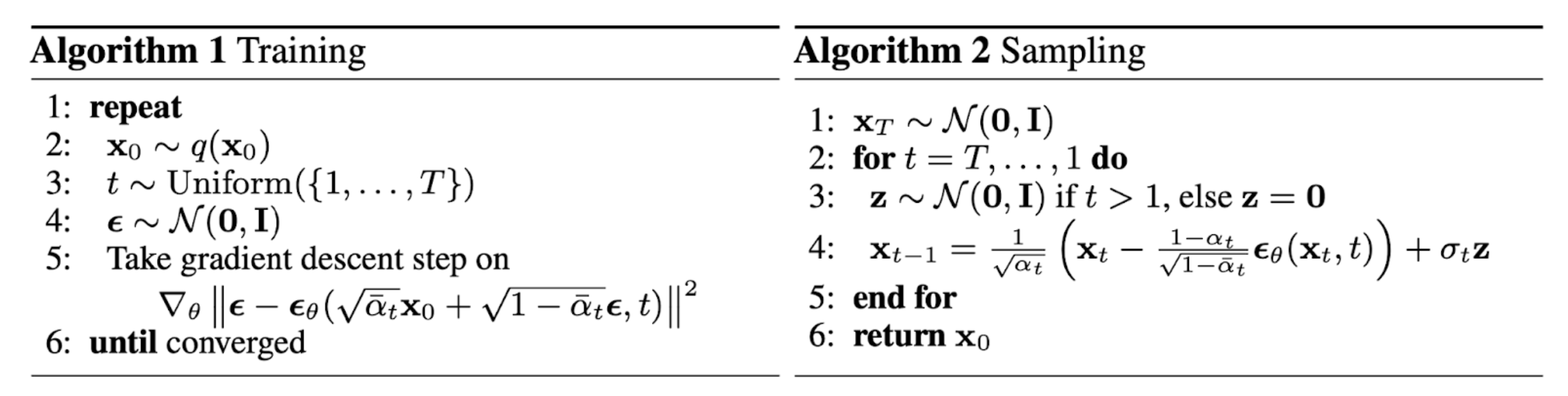 Fig. 4. The training and sampling algorithms in DDPM (Image source: Ho et al., 2020)
The neural network
U-Net, introduced by (Ronneberger et al., 2015), is a popular architecture for implementing noise predictors in diffusion models. Its efficiency and effectiveness have been demonstrated through its use in well-known diffusion-based models such as Stable Diffusion, Dall-E, Imagen, and Midjourney.
With the specific structure (U-shape), U-Net can learn meaningful spatial relationships between pixels in an image. For a more intuitive understanding, you can check out Sairam Sundaresan’s excellent blog post on the subject.
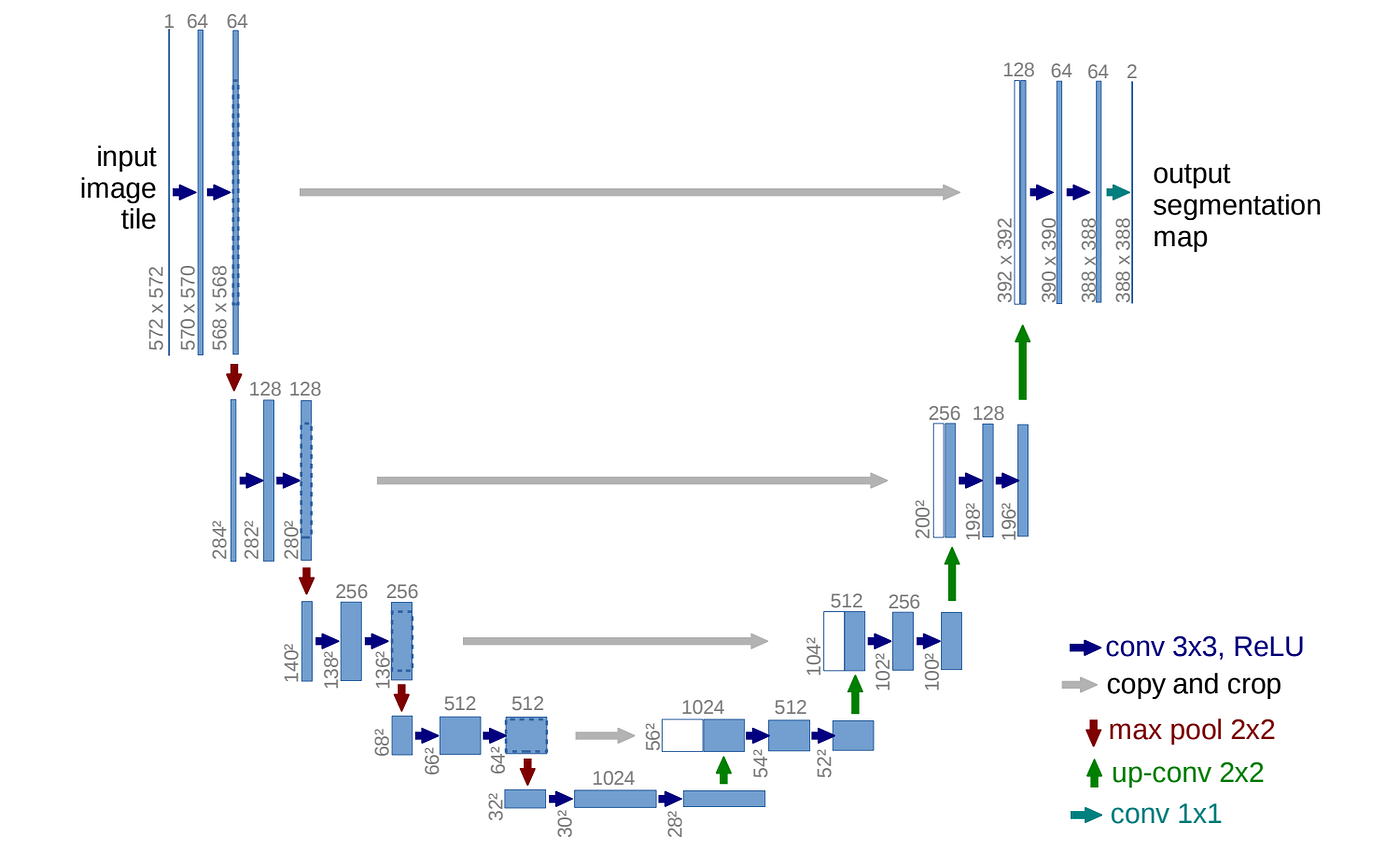 Fig 5. U-Net architecture (source: Ho et al., 2020)
Text-to-image synthesis
Text-to-image models need to be able to understand natural language descriptions in order to generate accurate and realistic images. Thus, text encoders are used to convert natural language descriptions into a format that can be understood by the model
Text encoder
Text encoders can be trained on paired text-image datasets (CLIP) or text-only datasets (BERT, GPT-4, T5, LLaMA). Those trained on paired text-image datasets are able to learn semantic and meaningful embeddings that are especially relevant for text-to-image synthesis. However, recent studies such as Imagen, Stable Diffusion have shown that large language models, which are trained on text-only datasets and have a deep understanding of natural language, can improve the quality of text-to-image synthesis.
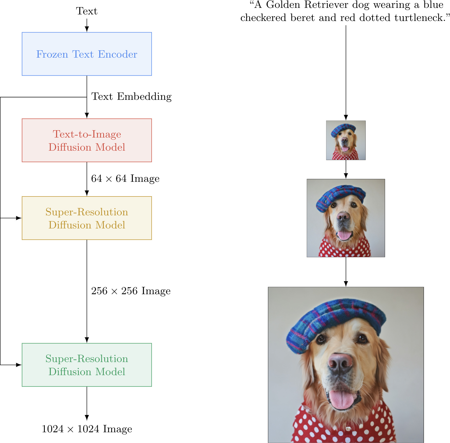 Fig 6. Imagen’s pipeline for Text-to-image synthesis (source: imagen)
Text conditioning
Like other generative models, diffusion models can be used to model conditional distributions, which means that they can be used to create new data that is conditioned on some input. To apply diffusion models to text-to-image synthesis, we can make them conditional by implementing them with a conditional denoising autoencoder \(\boldsymbol{\epsilon_\theta}(\mathbf{x}_t, t, \mathbf{y})\) and controlling the synthesis process through the conditioning \(\mathbf{y}\).
There are two ways to incorporate text conditioning into a neural network: by adding a text embedding to the diffusion timestep embedding or by using cross-attention. Both methods can also be combined for even better results. In the first method, we obtain a pooled text embedding vector from the text encoder and add it to the diffusion timestep embedding. In the second method, we use cross-attention over text embeddings at multiple resolutions to enhance the network’s understanding of the entire sequence of text embeddings. This helps the network generate more realistic images by better understanding the text.
Improvement techniques
In this blog post, I will discuss two effective methods for improving the quality of generated images and making the training process more efficient: Classifier-free guidance (CFG) and Exponential moving average (EMA).
The first method for enhancing the quality of output is Classifier-free guidance (CFG). Instead of using an independent classifier, CFG trains a single diffusion model on both conditional and unconditional objectives by randomly dropping the conditioning information \(\mathbf{y}\) during training. Hence, the adjusted denoising autoencoder becomes:
\[\begin{equation} \tilde{\boldsymbol{\epsilon}}_{\boldsymbol{\theta}} (\mathbf{x}_t, t, \mathbf{y}) = w\boldsymbol{\epsilon_\theta}(\mathbf{x}_t, t, \mathbf{y}) + (1 - w)\boldsymbol{\epsilon_\theta}(\mathbf{x}_t, t) \end{equation}\]The conditional and unconditional denoising autoencoders are respectively to \(\boldsymbol{\epsilon_\theta}(\mathbf{x}_t, t, \mathbf{y})\) and \(\boldsymbol{\epsilon_\theta}(\mathbf{x}_t, t)\), and the weight of the classifier-free guidance is denoted by $w$ in above equation.
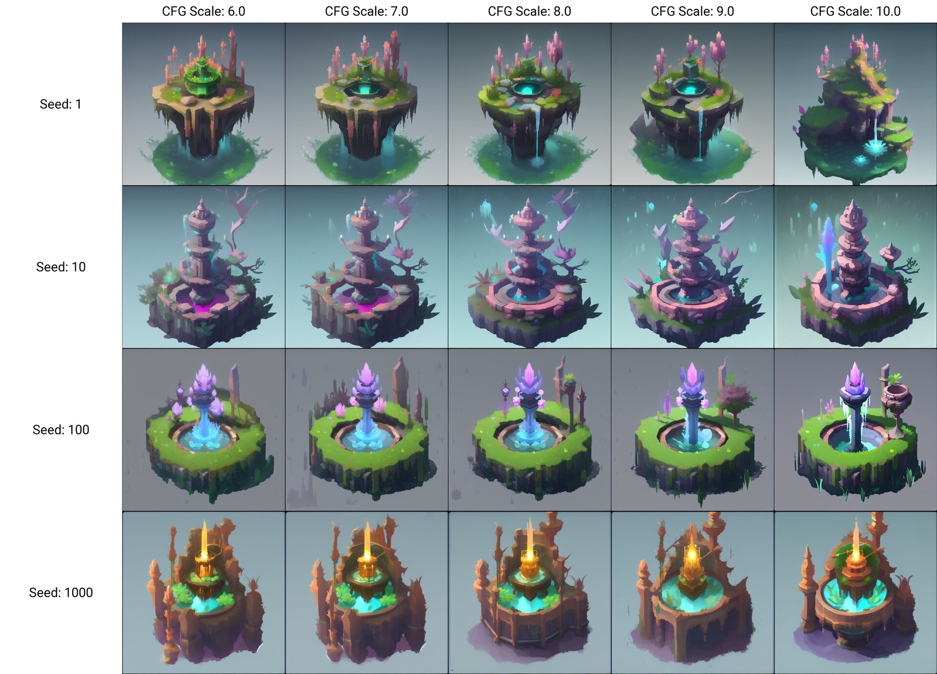 Fig 7. Higher CFG values results into more definition in shape and saturation (source: artstation)
The second method is Exponential moving average (EMA), which has been proven to enhance the stability and performance of diffusion models. It’s a straightforward technique that can improve the results of diffusion models by updating the model parameters through averaging over a certain number of steps.
References
- Ho, J., Jain, A., & Abbeel, P. (2020). Denoising Diffusion Probabilistic Models. arXiv [Cs.LG]. Retrieved from http://arxiv.org/abs/2006.11239.
- Weng, Lilian. “What Are Diffusion Models?”.
- Singh, Vaibhav . “An In-Depth Guide to Denoising Diffusion Probabilistic Models – from Theory to Implementation”.